4.9 Reasoning Behind the Growing Degree-Day Approximation
-
When a distinguished but elderly scientist states that something is possible, he is almost certainly right. When he states that something is impossible, he is very probably wrong.
-
The only way of discovering the limits of the possible is to venture a little way past them into the impossible.
-
Any sufficiently advanced technology is indistinguishable from magic (Clarke).
Given accurate and complete local daily temperature readings, we can predict codling moth development without relying on other observations (except, possibly, the first presence of adults at biofix). To be able to do this, we must magically approximate growing degree-days using just the daily maximum and minimum temperature.
Here is an examination of the behavior of the growing degree-day approximation, using real-world temperature data. This does not validate the codling moth development model against actual codling moth development over the years, but others have done so (U. C. Agriculture and Natural Resources, Research Models and Coop's Degree-Day Models).
4.9.1 Raw Data
Data consists of hourly automated instrumental temperature observations from the Sheboygan County, Wisconsin, Memorial Airport (KSBM) between 1996-08-31 18:53 and 2018-11-08 17:53. The precision appears to be about one degree Fahrenheit (ASOS-AWOS-METAR Data Download).
The numbers of observations are: 2694 (1996), 7954 (1997), 8587 (1998), 8207 (1999), 11094 (2000), 8657 (2001), 7915 (2002), 10969 (2003), 11563 (2004), 11181 (2005), 10946 (2006), 11401 (2007), 11942 (2008), 11578 (2009), 11368 (2010), 11581 (2011), 11155 (2012), 11786 (2013), 11714 (2014), 11334 (2015), 11709 (2016), 11456 (2017), and 9742 (2018).
There are several gaps of more than 5 hours. Many observations fall into these gaps and are not recorded. Some are recorded as missing. The numbers of gaps are: 4 (1996), 14 (1997), 4 (1998), 24 (1999), 18 (2000), 9 (2001), 12 (2002), 12 (2003), 10 (2004), 2 (2005), 19 (2006), 2 (2007), 3 (2008), 4 (2009), 1 (2010), 5 (2011), 2 (2013), 7 (2014), 4 (2015), 3 (2017), and 4 (2018). Taken together, these gaps cover many hours out of the years: 27 (1996), 140 (1997), 68 (1998), 427 (1999), 363 (2000), 99 (2001), 847 (2002), 249 (2003), 171 (2004), 13 (2005), 424 (2006), 17 (2007), 22 (2008), 32 (2009), 9 (2010), 110 (2011), 12 (2013), 110 (2014), 29 (2015), 95 (2017), and 111 (2018).
Now and then, there are runs of (at least 5) consecutive observations of identical temperature (in at least 5 hours), which I consider implausible. These represent malfunctions probably of hardware and more certainly of software and may be interpreted as attempts to "clean" the data by plugging in readings to conceal missing or out-of-range observations. I have taken the liberty of removing the days that such runs span:
1996-09-13, 1996-09-14, 1996-09-26, 1996-10-24, 1996-11-20, 1996-12-03, 1996-12-05, 1996-12-07, 1996-12-08, 1996-12-11, 1996-12-12, 1996-12-16, 1996-12-17, 1997-01-01, 1997-01-02, 1997-01-31, 1997-02-01, 1997-02-04, 1997-02-05, 1997-02-06, 1997-02-20, 1997-02-21, 1997-03-01, 1997-03-24, 1997-04-12, 1997-08-17, 1997-08-23, 1997-08-24, 1997-09-13, 1997-09-14, 1997-10-24, 1997-11-04, 1997-11-05, 1997-12-03, 1997-12-04, 1997-12-05, 1997-12-06, 1997-12-07, 1997-12-09, 1997-12-10, 1997-12-25, 1998-01-04, 1998-01-05, 1998-01-06, 1998-01-07, 1998-01-08, 1998-01-17, 1998-01-21, 1998-01-22, 1998-01-23, 1998-01-25, 1998-01-26, 1998-01-27, 1998-01-28, 1998-01-29, 1998-01-30, 1998-02-01, 1998-02-02, 1998-02-05, 1998-02-17, 1998-02-18, 1998-02-23, 1998-02-24, 1998-03-03, 1998-03-04, 1998-03-05, 1998-03-08, 1998-03-09, 1998-03-18, 1998-03-19, 1998-03-20, 1998-03-31, 1998-04-15, 1998-06-09, 1998-06-10, 1998-07-07, 1998-07-08, 1998-08-05, 1998-08-06, 1998-09-14, 1998-09-15, 1998-10-30, 1998-10-31, 1998-11-19, 1998-11-20, 1999-01-02, 1999-01-22, 1999-01-23, 1999-01-24, 1999-01-28, 1999-02-05, 1999-02-07, 1999-02-26, 1999-02-27, 1999-02-28, 1999-03-05, 1999-04-04, 1999-04-05, 1999-04-22, 1999-05-06, 1999-05-12, 1999-05-13, 1999-09-27, 1999-11-19, 1999-11-20, 1999-11-24, 1999-12-14, 1999-12-15, 2000-01-12, 2000-02-09, 2000-02-12, 2000-03-20, 2000-07-18, 2000-07-19, 2000-08-21, 2000-08-22, 2000-10-31, 2000-11-10, 2000-11-16, 2000-11-17, 2000-11-29, 2001-01-12, 2001-01-13, 2001-01-14, 2001-01-15, 2001-01-29, 2001-01-30, 2001-02-01, 2001-02-02, 2001-02-04, 2001-02-05, 2001-02-06, 2001-02-08, 2001-02-12, 2001-02-13, 2001-02-15, 2001-02-28, 2001-03-15, 2001-03-16, 2001-04-02, 2001-08-12, 2001-08-13, 2001-10-25, 2001-10-26, 2001-10-27, 2001-10-31, 2001-11-29, 2001-11-30, 2001-12-01, 2001-12-02, 2001-12-16, 2001-12-17, 2002-01-07, 2002-01-29, 2002-01-30, 2002-02-10, 2002-02-14, 2002-02-19, 2002-02-20, 2002-04-02, 2002-04-07, 2002-04-21, 2002-04-22, 2002-04-27, 2002-04-28, 2002-04-29, 2002-05-01, 2002-05-02, 2002-06-14, 2002-08-14, 2002-08-23, 2002-08-24, 2002-10-07, 2002-10-08, 2002-10-25, 2002-10-26, 2002-11-01, 2002-11-02, 2002-11-11, 2002-11-12, 2002-11-21, 2002-11-30, 2002-12-17, 2002-12-22, 2002-12-24, 2002-12-25, 2002-12-26, 2002-12-27, 2002-12-28, 2003-01-02, 2003-01-05, 2003-01-31, 2003-02-03, 2003-03-12, 2003-05-11, 2003-05-12, 2003-09-12, 2003-09-13, 2003-11-14, 2003-11-15, 2003-11-22, 2004-02-22, 2004-03-08, 2004-03-09, 2004-03-14, 2004-05-13, 2004-08-23, 2004-08-24, 2004-10-17, 2004-10-18, 2004-10-27, 2004-11-02, 2004-11-03, 2004-11-30, 2004-12-07, 2004-12-15, 2004-12-16, 2005-01-01, 2005-01-24, 2005-01-25, 2005-01-30, 2005-01-31, 2005-02-01, 2005-11-30, 2005-12-01, 2005-12-25, 2005-12-29, 2005-12-30, 2006-01-05, 2006-02-04, 2006-03-06, 2006-08-24, 2006-11-12, 2006-11-13, 2006-11-14, 2006-12-21, 2006-12-22, 2006-12-25, 2006-12-26, 2006-12-27, 2007-02-25, 2007-02-27, 2007-02-28, 2007-04-08, 2007-04-09, 2007-07-02, 2007-07-03, 2007-08-20, 2007-10-27, 2007-11-23, 2007-11-24, 2007-12-03, 2007-12-20, 2007-12-21, 2008-01-30, 2008-01-31, 2008-02-03, 2008-02-04, 2008-11-02, 2008-11-16, 2008-11-17, 2008-12-08, 2008-12-09, 2009-02-17, 2009-02-18, 2009-03-31, 2009-05-27, 2009-05-28, 2009-09-25, 2009-09-26, 2009-10-31, 2009-11-26, 2009-11-27, 2009-12-04, 2009-12-05, 2009-12-13, 2010-01-04, 2010-01-05, 2010-01-06, 2010-01-14, 2010-01-15, 2010-02-14, 2010-02-21, 2010-02-28, 2010-03-12, 2010-08-04, 2010-09-11, 2010-12-18, 2010-12-19, 2011-01-19, 2011-01-27, 2011-01-28, 2011-03-01, 2011-03-09, 2011-05-03, 2011-11-27, 2011-12-16, 2012-03-30, 2012-03-31, 2012-04-19, 2012-04-20, 2012-10-14, 2012-10-29, 2012-10-30, 2012-11-09, 2012-11-10, 2012-11-30, 2012-12-12, 2012-12-26, 2012-12-27, 2012-12-28, 2013-01-03, 2013-01-16, 2013-02-01, 2013-02-09, 2013-03-23, 2013-03-24, 2013-06-05, 2013-06-06, 2013-07-02, 2013-07-03, 2013-07-18, 2013-07-19, 2013-10-03, 2013-10-04, 2013-11-27, 2013-11-28, 2013-12-03, 2013-12-04, 2013-12-20, 2013-12-21, 2013-12-30, 2013-12-31, 2014-01-09, 2014-01-10, 2014-01-11, 2014-01-20, 2014-01-30, 2014-02-17, 2014-03-19, 2014-04-03, 2014-04-23, 2014-04-24, 2014-06-10, 2014-08-21, 2014-08-22, 2014-08-23, 2014-08-24, 2014-09-11, 2014-09-12, 2014-09-13, 2014-10-14, 2014-10-15, 2014-10-20, 2014-10-21, 2014-10-31, 2014-11-01, 2014-11-05, 2014-12-08, 2014-12-09, 2014-12-10, 2014-12-12, 2014-12-13, 2014-12-20, 2014-12-21, 2014-12-24, 2014-12-25, 2014-12-31, 2015-01-12, 2015-01-13, 2015-01-14, 2015-01-15, 2015-01-20, 2015-01-27, 2015-02-04, 2015-02-08, 2015-02-16, 2015-02-17, 2015-03-25, 2015-03-26, 2015-08-25, 2015-08-26, 2015-10-03, 2015-10-04, 2015-10-05, 2015-10-06, 2015-11-27, 2015-11-30, 2015-12-21, 2015-12-22, 2015-12-26, 2015-12-30, 2016-01-03, 2016-01-06, 2016-01-07, 2016-01-21, 2016-01-25, 2016-02-04, 2016-02-14, 2016-02-18, 2016-02-19, 2016-02-21, 2016-02-22, 2016-02-25, 2016-03-21, 2016-05-10, 2016-05-11, 2016-07-04, 2016-07-05, 2016-07-20, 2016-07-21, 2016-08-07, 2016-08-12, 2016-08-13, 2016-09-07, 2016-10-01, 2016-10-02, 2016-10-26, 2016-11-16, 2016-11-17, 2016-11-23, 2016-11-25, 2016-11-30, 2016-12-01, 2016-12-02, 2016-12-03, 2016-12-04, 2016-12-10, 2016-12-17, 2016-12-24, 2017-01-02, 2017-01-03, 2017-01-05, 2017-01-06, 2017-01-17, 2017-01-18, 2017-01-24, 2017-01-26, 2017-01-27, 2017-02-11, 2017-02-12, 2017-02-24, 2017-03-04, 2017-03-05, 2017-03-24, 2017-03-25, 2017-03-26, 2017-03-30, 2017-03-31, 2017-04-17, 2017-04-18, 2017-05-02, 2017-08-06, 2017-08-07, 2017-10-12, 2017-10-13, 2017-10-14, 2017-11-04, 2017-11-05, 2017-11-11, 2017-11-15, 2017-11-16, 2017-11-18, 2017-12-05, 2017-12-06, 2017-12-07, 2017-12-10, 2017-12-12, 2017-12-13, 2017-12-16, 2017-12-17, 2017-12-18, 2017-12-28, 2018-01-17, 2018-01-18, 2018-01-22, 2018-01-24, 2018-02-07, 2018-02-22, 2018-03-08, 2018-04-03, 2018-04-08, 2018-04-09, 2018-04-13, 2018-04-14, 2018-05-19, 2018-09-20, 2018-09-28, 2018-10-13, 2018-10-14, 2018-11-06.
The days in boldfaced text occur within months that contain (at least 3) corrupt days.
Because I plan to use this data to conduct sensitivity analysis of the model for codling moth development, I need to have fairly complete summer records. Accordingly, I have removed some years altogether that contain corrupt summer months: 2013, 2014, 2016.
I searched for discontinuities in the data that remains with a moving window of (5) observations. I tried to predict the next observation by running a trend line through the window. I examined each discontinuity where my prediction differed from the actual by more than 20°F.
Upon inspection, many of these discontinuities appeared plausible. Others appeared after data gaps. I took the liberty of eliminating a number observations that appeared implausible: 4 on 1996-10-01, 4 on 1997-05-01, 5 on 1997-12-01, 6 on 1998-01-01, 6 on 1998-12-01, 6 on 1999-01-01, 6 on 1999-03-01, 6 on 1999-05-01, 6 on 1999-11-01, 2 on 2000-11-03, and 1 on 2001-07-31. That these rejected observations were taken on the first day of the month in many cases is curious.The numbers of discontinuities remaining are: 3 (1996), 17 (1997), 13 (1998), 20 (1999), 13 (2000), 9 (2001), 11 (2002), 8 (2003), 12 (2004), 5 (2005), 7 (2006), 5 (2007), 4 (2008), 4 (2009), 8 (2010), 6 (2011), 4 (2012), 7 (2015), 13 (2017), and 11 (2018).
4.9.2 Daily Average Temperature
The first thing to do is show what average temperatures look like over 24 hours during the summer. Here is a spaghetti plot where each thread is a day in July and August.
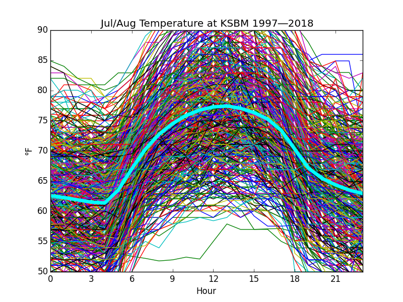
Fig. A
The belief that temperature is a continuous phenomenon is compelling, and the lacy appearance of the spaghetti plot shown in Fig. A is disturbing because it shows that temperatures are clustered. This is because temperature is recorded in whole degrees Fahrenheit and on hourly intervals; nevertheless, because the underlying phenomenon must be continuous, there should be no particular intellectual difficulty in making the statistical leap of faith that we can treat the discrete measurements as though they are, too.
Thus, the curve highlighted in light blue can be said fairly to represent the average from hour to hour of summer temperatures. Note that it is skewed slightly toward the afternoon.
The next step is to idealize this curve. Here is the same spaghetti plot overlaid by an ideal sine wave.
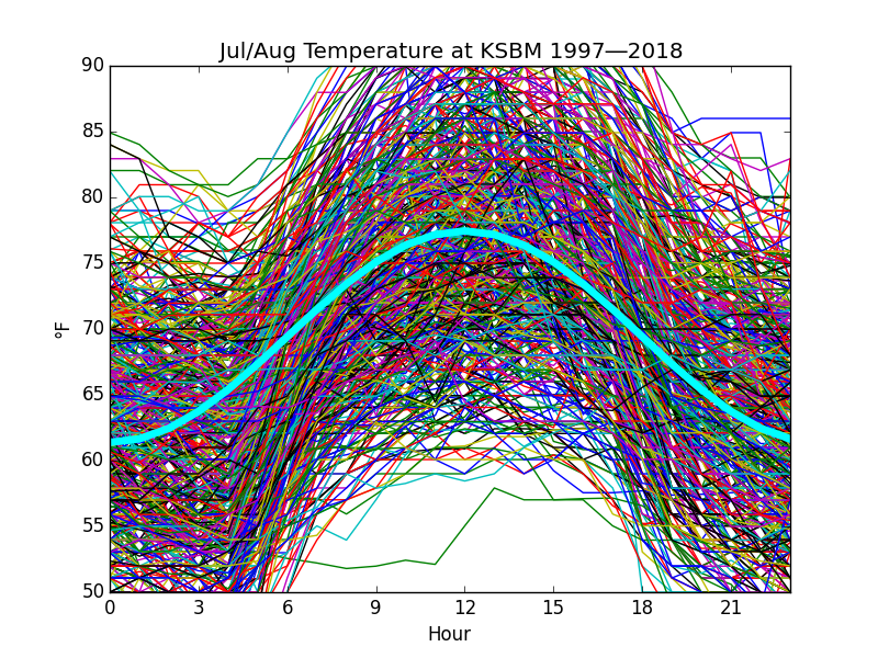
Fig. B
This ideal curve shown in Fig. B closely matches the actual shown in Fig. A except for the skew and will be the basis for arguments that follow. By characterizing hourly temperatures during a day as a sine wave, the temperature at any hour does not have to be measured and recorded. Instead, an approximation can be calculated, given the maximum and minimum temperatures for that day. Also, the sine has pleasant mathematical properties that make some of the anticipated calculations fairly easy to do.
... so what should we do with this ideal curve? Plot growing degree-days, of course.
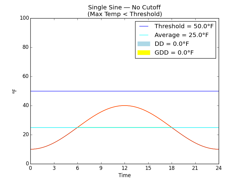
Fig. C
Fig. C shows how the temperature may vary during a chilly day. The daily maximum temperature is below the threshold temperature at which insect development begins, so there can be no growing degree-days accrued at all for this day.
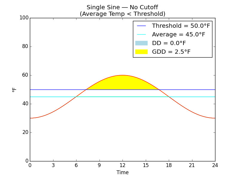
Fig. D
Fig. D shows a warmer day when the daily maximum temperature crosses the threshold temperature for a portion of the day. On a day such as this, we would record a small amount of growing degree-days (GDD).
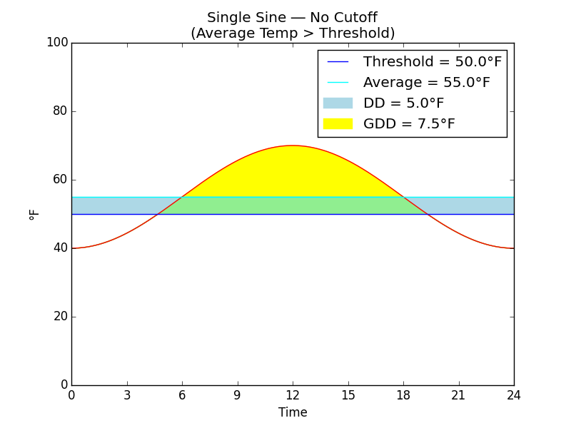
Fig. E
Fig. E shows a still warmer day when not only the daily maximum temperature crosses the threshold but also the daily average temperature is above the threshold. On a day like this, we would record a larger amount of growing degree-days, shown in yellow and green. Also, the conventional way of calculating degree-days (DD), which is the difference shown in green and blue between the average temperature and the threshold, is positive but not so large as the growing degree-days. The average temperature is assumed to be:
\begin{equation} TAvg = (TMax + TMin) / 2.0 \end{equation}\begin{equation} \label{dd} DD = TAvg - TThreshold \end{equation}
... where \(TMax\) is maximum daily temperature and \(TMin\) is minimum daily temperature. For this reason the conventional DD calculation is sometimes called the max-min method. Note that both DD and GDD are constrained not to be negative.
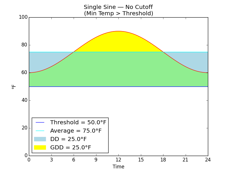
Fig. F
Fig. F shows a succession of warm nights when the daily minimum temperatures are above the threshold. Over a 24-hour period such as this, the growing degree-days, shown in yellow and green, is identical to the conventional degree-days, shown in green and blue.
The rationale for using the sine wave instead of the max-min average is this: By using the sine wave, we can capture more days on which there is a small contribution to insect development even though the average temperature is below the threshold.
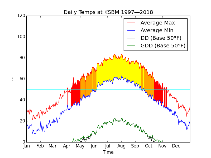
Fig. G
Returning to the actual data for Sheboygan, Fig. G shows the average daily maximum and minimum temperatures recorded. Also shown are the conventional degree-days (DD) and the growing degree_days (GDD). Yellow highlights the days when daily minimum is above the threshold. On these days, DD and GDD track together. Orange highlights the days when DD and GDD diverge. Red highlights the days when only GDD is accrued. Thus, in Sheboygan the accrual of GDD begins earlier and thus outruns the accrual of DD for a period of six weeks in the spring.
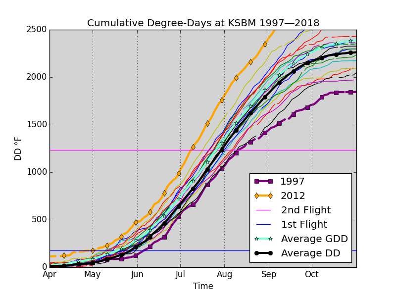
Fig. H
Fig. H shows a spaghetti plot of the cumulative GDD in Sheboygan where each thread is a different year. 2012 was the warmest. 1997 was the coldest.
It is tempting to make too much of the year-to-year temperature trend and point to this as evidence of climate change brought about by anthropogenic global warming (AGW). There are several problems:
The raw data is collected at an airport without commercial passenger service. The purpose of this automated data collection is to support fixed base operations (FBO) at that airport, which relays near current conditions to pilots via radio and telephone. The data items of primary interest are wind speed and direction, visibility, and precipitation. The motivation for collecting and disseminating the data is for immediate consumption. Because the audience considers the data ephemeral, no particular care is taken to be sure the archived temperature record is precise, accurate, or even complete. Thus, it is a misuse of the data to make historical comparisons as I have done.
Further, I have made the comparisons while avoiding dealing with incomplete records. The gaps are apparent in the 1997 plot line. Thus, no GDD accrual is made on the days for which no plausible temperature information exists even though there ought to have been some accrual, and the curve as drawn turns out to be lower than the actual curve should have been, had all days been taken into account. I studied statistics briefly, including notions about how to keep track of statistical error, and was taught that, while it may be possible to combine data sources to fill gaps and while it may be possible in some circumstances to posit models of the data from which gaps may be artificially filled, these techniques do not reduce error but magnify it, and I have attempted no such thing. I can point to obvious flaws in my rendition, but I would rather do that than present something superficially truer that differs from fact in ways that are more difficult to explain.
The Sheboygan County Memorial Airport is a larger facility today than it was 20 years ago with longer runways and much more hangar space under roof. It is too much to expect that daily temperature fluctuations at the site would remain completely unaffected by the development.
The cumulative growing degree-days in 2012 was at least 2888°F. In 1997, it was at least 1849°F. The difference is 1039°F, which would represent daily temperatures 2.8°F (1.9°C) higher. I don't know of any claims that AGW amounts to that much. This is variability, not necessarily trend.
Finally, we ought to give lip service to what climate is. Climate change is, by definition, long-term fluctuation in prevailing weather over time scales beyond living memory. Climate change is not your granddad telling you about meager crops during the Dust Bowl years. Climate change is collapse of the Mississippian Culture, the Tiwanaku Civilization around Lake Titicaca in present-day Bolivia, and the Ancestral Puebloan Culture in the three centuries between 1130 and 1430 AD (Wikipedia, Ancestral Puebloans).
Climate change is Calvin Coolidge's promoting the idea at the Minnesota State Fair of 1925 that Vikings discovered America around 1000 AD (Wikipedia, "Leif Erikson Day"). Although this was backed by Icelandic literary tradition, he asserted it in spite of the utter absence of any archaeological evidence (which has since come to light). Greenland was colonized in 985 AD during the Medieval Warm Period (MWP) by Icelandic real-estate speculator Erik "the Red" Thorvaldsson. His son, Leif Erikson, was the first and only Christian to visit the North American continent beyond Greenland before Italian real-estate speculator Christopher Columbus managed it during the depths of the Little Ice Age (LIA), which followed. The Greenland colonies, like many of the pueblos of the American Southwest, were abandoned sometime in the early 1400s (Fritz).
4.9.3 Variability
"Over the Mountains
Of the Moon,
Down the Valley of the Shadow,
Ride, boldly ride,"
The shade replied—
"If you seek for Eldorado (1849, Poe)!"
Fig. H shows a spaghetti plot of the cumulative GDD in Sheboygan along with the two prominent horizons of codling moth development: the first and second flight. For a given year, the time of a flight is predicted by when the cumulative GDD curve crosses the respective horizon. From the warmest (earliest) year to the coolest (latest) year, the difference between the dates of the first flight can be as much as five weeks and the same for the second flight.
Two successive chemical treatments ten days apart will suppress larval activity for at most three weeks. Thus, chemical control cannot span the natural variability in the dates of codling moth development.
For this reason it is better not to rely on a calendar for timing codling moth treatment. That is what the ancient Egyptians did who tried to predict the snow melt on the Mountains of the Moon. For timing codling moth treatment it is better to rely on tracking cumulative growing degree-days using the methods proposed by Baskerville and Emin.
4.9.4 Methods of Calculation
Fig. H shows a spaghetti plot of the cumulative GDD in Sheboygan along with the average cumulative GDD and the average cumulative conventional DD. The growing degree-days (GDD) calculated by Baskerville and Emin's single sine horizontal cutoff method outruns the conventional degree-days (DD) calculated by the max-min method by about a week. Thus, for timing codling moth treatment, the method used to calculate degree-days is significant, and methods calculating growing degree-days rather than conventional degree-days are preferred.
There are other methods of estimating growing degree-days besides single sine. U. C. Agriculture and Natural Resources (UCANR) publishes on their Web site a discussion of "Degree-Days," which describes similar methods. Also, they publish an "Evaluation of Several Degree-Day Estimation Methods in California Climates," which reviews performance of single sine, double sine, single triangle, and double triangle methods (among others) against hourly summation and concludes that all methods yield similar results during the spring and summer and that there is no particular advantage of the doubled methods that treat morning and afternoon separately. "The single triangle and single sine methods estimate degree-days relativity well," they say. While single triangle may be superior during the fall and winter (for daily temperature patterns experienced in California), use of single sine is still customary for studies of insect development.
Much of the research validating insect development against growing degree-days recommends single sine methods (UCANR, "Research Models"), but many papers apparently do not specify the method by which their authors arrived at growing degree-days. This leads one to conclude that any of the practical methods for estimating growing degree-days are probably adequate.
4.9.4.1 Single Sine
Coop presents a computer algorithm for calculating growing degree-days. Here's how it works. Temperatures are assumed to follow an idealized sine wave throughout the hours of each day. The sine wave is clipped horizontally from below by the threshold temperature. Growing degree-days for each day is proportional to the area under the curve above the threshold, which thus depends on the threshold and the maximum and minimum temperatures for each day.
The algebra, trigonometry, and Integral Calculus involved are apparently not too exotic but are fairly obscure. Here follows my reconstruction.
If the threshold temperature is below the daily minimum temperature, the answer we must give is the conventional one. See Formula \(\ref{dd}\), above. This is because the curve is not clipped.
Below, we're going to use the following ¨simplifying¨ expression, so I suppose I ought to define it here.
\begin{align} Let \quad D2& = -2 * DD\\ & = 2 * TThreshold - (TMax + TMin) \end{align}
Consider a sine wave from \(-\pi/2\) to \(3\pi/2\) radians with its peak at high noon (\(\pi/2\) radians).
If the threshold temp is above the daily minimum temp, we need to integrate over a portion of the curve. The essential magic is to discover the angle \(\Theta\) where the sine wave, scaled and offset to the average temperature, crosses this threshold. Then we can cast away the area below the threshold along with the tails of the curve.
Because the sine wave is symmetric about \(\pi/2\), we need to integrate only between \(-\pi/2\) and \(\pi/2\).
The definite integral of the sine wave from \(-\pi/2\) and \(+\pi/2\) is zero because half of it is negative, so that doesn't do us much good. We'll have to choose a different function. How about \(\sin + 1\)?
\begin{align} \int_{-\pi/2}^{+\pi/2}{(\sin(t) + 1)}dt& = -\cos(\pi/2) - (-\cos(-\pi/2)) + \pi/2 - (-\pi/2)\\ & = \pi \end{align}
This is the area under the curve. To normalize the calculations to follow, we have to multiply by this:
\begin{equation} DownscaleFactor = 1 / \pi \end{equation}
When \(TThreshold == TMin\) and \(\Theta == -\pi/2\), the answer we must give is \(DD\) as in Formula \(\ref{dd}\). This becomes our upscale_factor:
\begin{align} UpscaleFactor& = ((TMax + TTMin) / 2) - TThreshold\\ & = (TMax + TMin - 2 * TThreshold) / 2\\ & = (TMax + TMin - 2 * TMin) / 2\\ & = (TMax - TMin) / 2 \end{align}
The following formula is similar to that given by Baskerville and Emin in their Fig. 1.B:
\begin{equation} GDD = DownscaleFactor * (UpscaleFactor * WholeArea - ClippedArea))\\ \end{equation}
where:
\begin{align} WholeArea& = \int_{\Theta}^{\pi/2}{(sin(t) + 1)}dt\\ & = -\cos(\pi/2) - (-\cos(\Theta)) + (\pi/2 - \Theta)\\ & = \cos(\Theta) + (\pi/2 - \Theta) \end{align}
\begin{align} ClippedArea& = \int_{\Theta}^{\pi/2}{(TThreshold - TMin)}dt\\ & = (TThreshold - TMin) * (\pi/2 - \Theta) \end{align}
thus:
\begin{multline} GDD = DownscaleFactor * (UpscaleFactor * (\cos(\Theta)\\ + (\pi/2 - \Theta))) - (TThreshold - TMin) * (\pi/2 - \Theta) \end{multline}\begin{multline} \quad = (1 / \pi) * (((TMax - TMin) * (\cos(\Theta)\\ + (\pi/2 - \Theta)) / 2) - ((TThreshold - TMin) * (\pi/2 - \Theta))) \end{multline}\begin{multline} \quad = (1 / 2\pi) * ((TMax - TMin) * (\cos(\Theta)\\ + (\pi/2 - \Theta)) - 2 * (TThreshold - TMin) * (\pi/2 - \Theta)) \end{multline}\begin{multline} \quad = (1 / 2\pi) * ((TMax - TMin) * \cos(\Theta)\\ + (TMax - TMin) * (\pi/2 - \Theta) - 2 * (TThreshold - TMin) * (\pi/2 - \Theta)) \end{multline}\begin{multline} \quad = (1 / 2\pi) * ((TMax - TMin) * \cos(\Theta)\\ + ((TMax - TMin) - 2 * (TThreshold - TMin)) * (\pi/2 - \Theta)) \end{multline}\begin{multline} \quad = (1 / 2\pi) * ((TMax - TMin) * \cos(\Theta)\\ + (TMax - TMin - 2 * TThreshold + 2 * TMin) * (\pi/2 - \Theta)) \end{multline}\begin{multline} \quad = (1 / 2\pi) * ((TMax - TMin) * \cos(\Theta)\\ + (TMax - 2 * TThreshold + TMin) * (\pi/2 - \Theta)) \end{multline}\begin{multline} \quad = (1 / 2\pi) * ((TMax - TMin) * \cos(\Theta)\\ - (2 * TThreshold - (TMax + TMin)) * (\pi/2 - \Theta)) \end{multline}\begin{multline} \quad = (1 / 2\pi) * ((TMax - TMin) * \cos(\Theta) - D2 * (\pi/2 - \Theta)) \end{multline}
... which is the formula that Coop uses to calculate GDD.
=====
QED
=====
Now, for the essential magic we need to compute:
\begin{equation} \label{arcsin} \Theta = \arcsin(UnitBase) \end{equation}
... where \(UnitBase\) is the threshold temperature scaled to the sine wave (not \(\sin + 1\)):
\begin{multline} UnitBase = 2 * (TThreshold - TMin) / (TMax - TMin) - 1 \end{multline}\begin{multline} \quad = (2 * (TThreshold - TMin) - (TMax - TMin)) / (TMax - TMin) \end{multline}\begin{multline} \quad = (2 * TThreshold - 2 * TMin - TMax + TMin) / (TMax - TMin) \end{multline}\begin{multline} \quad = (2 * TThreshold - TMin - TMax) / (TMax - TMin) \end{multline}\begin{multline} \quad = (2 * TThreshold - (TMax + TMin)) / (TMax - TMin) \end{multline}\begin{multline} \quad = D2 / (TMax - TMin) \end{multline}
But there's a fly in this ointment. We want to have pretty good computational accuracy where \(UnitBase\) is pretty close to \(\pm1\), which should yield an \(\arcsin\) result pretty close to \(\pm\pi/2\), but that is just where the accuracy of real-world \(\arcsin\) implementations falls down due to inherent granularity of simulating mathematics of continuous functions on binary machines, which can handle only discrete values.
Maybe it would be better to calculate \(\Theta\) using the \(\arctan\), instead.
I think it's just this easy:
\(\sin(\Theta) = a / c\) where the sides of the right triangle are:
\((a * a) + (b * b) = (c * c)\)
and, using the same angle:
\(\tan(\Theta) = a / b = a / \sqrt{c^2 - a^2}\)
\begin{equation} Now \quad \Theta = \arcsin(a / c) \end{equation}
and by Formula \(\ref{arcsin}\) this means that:
\begin{align} a& = UnitBase\\ and \quad c& = 1 \end{align}
Then, the same angle would be:
\begin{align} \Theta& = \arctan(a / \sqrt{c^2 - a^2})\\ & = \arctan(UnitBase / \sqrt{(1 * 1) - (UnitBase * UnitBase)})\\ & = \arctan((D2 / (TMax - TMin)) / \sqrt{1 - (D2 / (TMax - TMin))^2})\\ & = \arctan(D2 / \sqrt{(TMax - TMin) * (TMax - TMin) - D2 * D2}) \end{align}
... which, if I have not deluded myself, is the formula for \(\Theta\) used by Coop. (In practice however, using the \(\arcsin\) yields identical results rounded to the nearest integer.)
Nowadays, we are accustomed to enjoying the fruits of high-speed computing and think nothing of writing little programs to churn through thousands of such calculations that would have been extremely tedious, time consuming, and error prone to work out with a slide rule. The ease with which it is done causes us to imagine that, however minuscule the improvement in timing insect treatments, the effort is small and will surely be repaid.
4.9.4.2 Cutoff
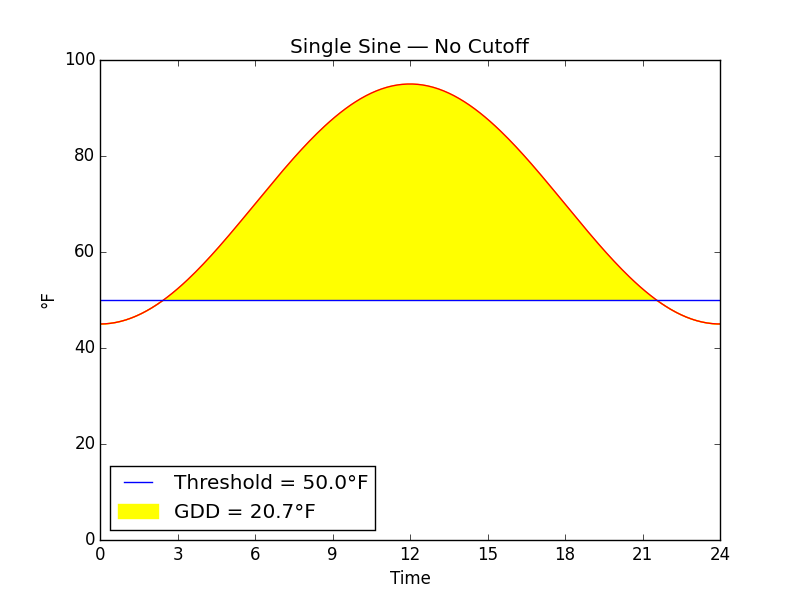
Fig. I
Fig. I shows growing degree-days without any cutoff.
The lower threshold is implicit in the single sine method. Obviously insect development slows in cooler weather. The lower threshold preserves the proportionality of insect development with growing degree-days by introducing non-linearity between temperature and growing degree-days. It is to be expected that some kind of upper cutoff is required, as well. Baskerville and Emin demonstrate two approaches.
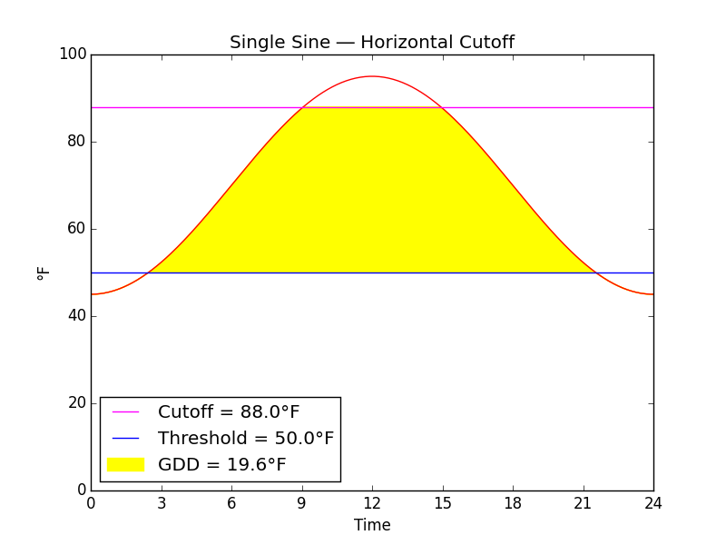
Fig. J
Fig. J shows the horizontal cutoff typical of the codling moth model and other insect models.
In warm weather, insect development is not constrained by temperature, which is to say it is constrained by other things and no longer dependent on temperature. To preserve proportionality of insect development with growing degree-days, it is necessary to introduce non-linearity between temperature and growing degree-days at warmer temperatures. One way to achieve this is with a horizontal cutoff.
Once we are able to characterize the formula for growing degree-days without any cutoff in terms of just \(TMax\), \(TMin\), and \(TThreshold\), it is trivial to characterize the area to be "cutoff" with the same formula in terms of just \(TMax\), \(TMin\), and \(TCutoff\).
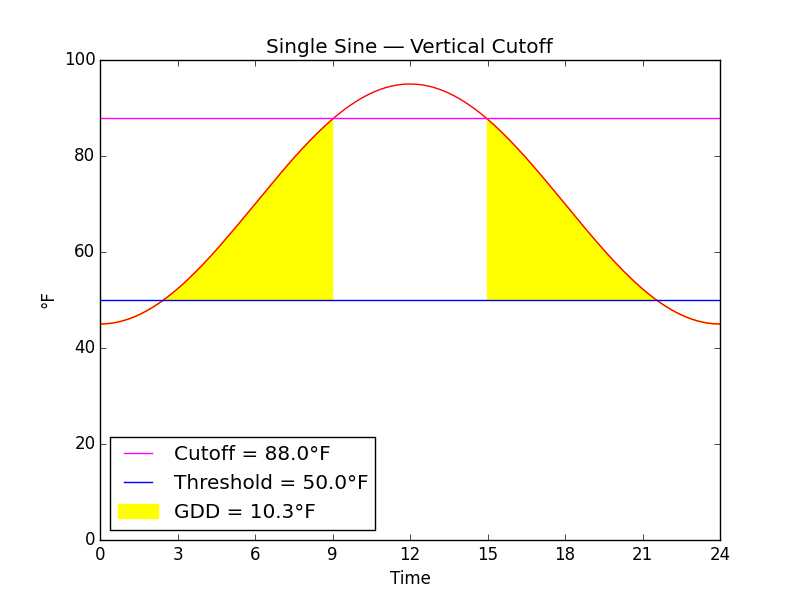
Fig. K
Fig. K shows a vertical cutoff, which is not typical of the model for Codling Moth although it is typical of other insects such as Spotted Tentiform Leafminer (Phyllonorycter blancardella).
In warm weather, insect development may be slowed or stopped just as it is in cool weather. Another way to introduce non-linearity between temperature and growing degree-days at warmer temperatures is with a vertical cutoff,
We can characterize the area to be "cutoff" as the same as the horizontal cutoff plus the rectangle beneath it.
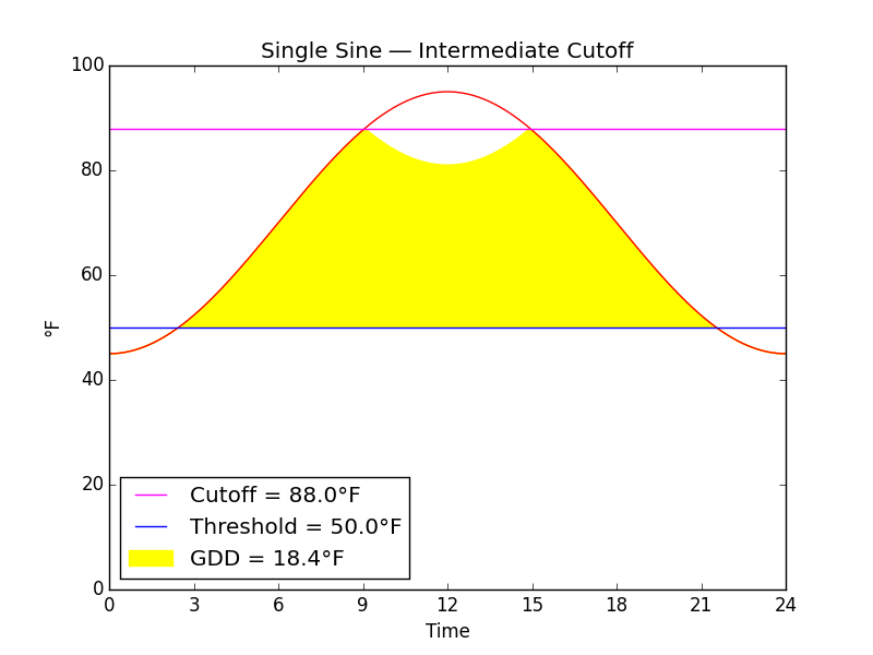
Fig. L
Fig. L shows a cutoff intermediate between a horizontal and a vertical cutoff. The intermediate cutoff has been validated for Blue Alfalfa Aphid (Acyrthosiphon kondoi).
The intermediate cutoff was not demonstrated by Baskerville and Emin, but it is easily implemented. It is double the area of the horizontal cutoff.
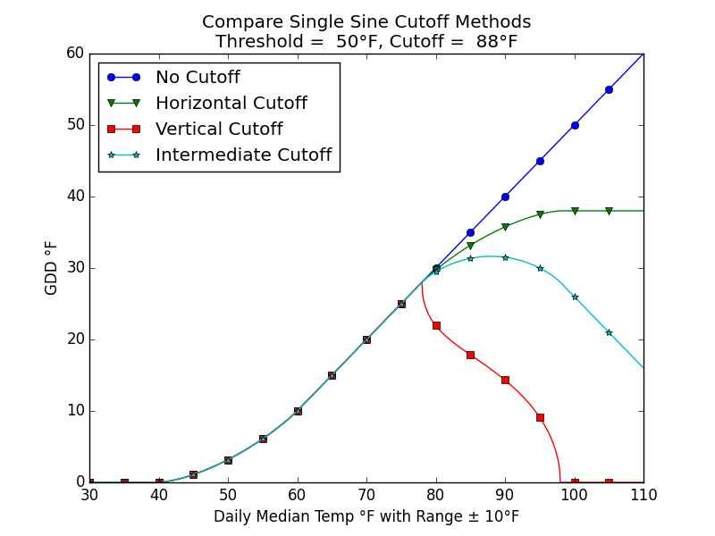
Fig. M
Fig. M compares the behavior of the three kinds of cutoff against temperature. All of the sine methods show a flattening of growing degree-days with decreasing temperature at the threshold. The same is to be expected at the cutoff. Without a cutoff, growing degree-days and insect development would increase indefinitely with increasing temperature, and this is implausible. The horizontal cutoff gives the same kind of flattening at the cutoff temperature that all methods exhibit at the threshold temperature. Thus, it is useful for modeling the insects whose development plateaus in warm weather. The vertical cutoff is for insects that show an abrupt decrease in development at the cutoff temperature, and the intermediate cutoff is better for insects that show a more graceful decline.
Naturally, the reader is encouraged to seek out research that validates growing degree-day models for the insect species to be treated. (See, for example, the list of insect "Research Models" published by U. C. Agriculture and Natural Resources, and please refer to Coop's "Library of Degree-Day Models," as well.) The reader should expect to gain an inkling of the calculation method and kind of cutoff used by the researchers. In the absence of these, it is not unreasonable to choose single sine with horizontal cutoff. More importantly, the research ought to indicate the threshold and cutoff temperatures that govern the development of the species to be treated.
4.10 What Can Go Wrong
But, Mousie, thou art no thy-lane,
In proving foresight may be vain;
The best-laid schemes o' mice an' men
Gang aft agley,
An' lea'e us nought but grief an' pain,
For promis'd joy!
Still thou art blest, compar'd wi' me
The present only toucheth thee:
But, Och! I backward cast my e'e.
On prospects drear!
An' forward, tho' I canna see,
I guess an' fear (1785, Burns)!
The growing degree-day model of codling moth development described, above, is remarkably immune to small random errors in measuring daily maximum and minimum temperatures and can be counted on to give reasonable results with casual use, but a number of things still can go wrong.
4.10.1 Microclimate
One thing that can go wrong is consistent error in recording daily maximum and minimum temperatures. This is likely to occur if the orchard has been planted in a microclimate where prevailing temperatures may diverge significantly and consistently from those reported by the nearest weather station.
For example, an offshore breeze near a large inland lake will not change temperatures drastically, but an onshore breeze lowers them as much as 10°F in the spring. Thus, even if wind direction were completely random, the actual daily temperatures would be biased much lower overall than those reported only a few city blocks further inland. Growing degree-days calculated with reported temperatures would thus outrun those calculated with actual temperatures.
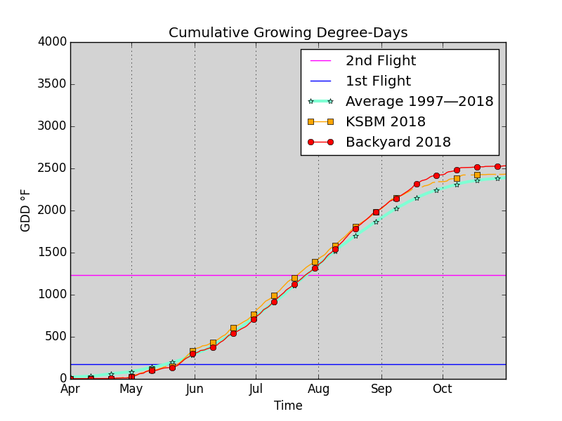
Fig. N
Fig. N shows how microclimate affects cumulative growing degree-days. In 2018, I was able to capture daily maximum and minimum temperatures in my backyard, using weeWX software to manage an Ambient Weather WS-2095 Wireless Home Weather Station. The red curve is is calculated from these readings taken two blocks from Lake Michigan. The Sheboygan County Memorial Airport (KSBM) is located seven miles inland from Lake Michigan. The orange curve is calculated from automated instrumental temperature observations taken there. The cumulative growing degree-days at the airport outran the cumulative growing degree-days at my home beginning in late May. The predicted date of the codling moth second flight in July was four or five days earlier using airport data.
Although the first flight predicted by the airport data and that predicted by the backyard data were within a day of one another, the airport reached the egg-hatching stage by accumulating 250 growing degree-days in in 16 days, whereas my backyard weather station required 20 days.
The cumulative growing degree-days at my home outran the cumulative growing degree-days at the airport beginning in August. There are obvious gaps in the airport records, which cause the cumulative growing degree-days to be lower than they ought to be. Another justification for the backyard data's outrunning the airport data may be that the lake exerts a warming effect in the fall. It is often remarked that, although we do without spring in Sheboygan, our autumn goes on forever. It may also be that the heat-island effect produced by the city is more prominent in my backyard in the fall as the relatively warmer water of the lake draws a persistent off-shore breeze.
The obvious solution to microclimate bias at public weather-reporting stations is to use actual temperatures recorded by a miniature backyard weather station.
There are other kinds of microclimates. Downhill and uphill breezes in mountainous locations may cool and heat areas exposed to them while protected areas are not so susceptible. Even the slope of an orchard toward or away from the sun affects the prevailing temperature in hilly locations.
Urban heat islands are a prevalent type of microclimate. Modification of land surfaces in cities captures solar energy, which warms the air at ground level particularly after dark (Wikipedia, Urban Heat Island). Waste heat from human activity is also a factor. The combined effect can be as much as 5°F. Official weather reporting stations may or may not be located within urban heat islands. Nearly all reports of prevailing temperature are affected by urban heat islands because most gardeners either live in an urban heat island or rely on reports from inside one. Certainly wind direction plays a part with actual temperatures biased much higher overall.
To repeat: Daily maximum and minimum temperatures used in the model to predict codling moth development and plan control strategies must be taken as close to the orchard as possible -- preferably within it -- in order to eliminate microclimate bias.
4.10.2 Miscalibration
Another source of consistent error is miscalibration of temperature-measuring equipment. Growing degree-day models are based on accumulated environmental heating, and consistent errors in measurement build up during the hundred or so days in a season.
4.10.3 Fuzzy Biofix
The attractive aspect of the codling moth development model is its objectivity. Development seems to depend completely and only upon growing degree-days. This is an illusion, however. The critical decision is where to place the biofix because this affects the timing of all the subsequent applications of chemical controls. Determining the biofix becomes somewhat subjective when inclement weather splits the first flight into two or more "cohorts."
A cohort in this situation is a group of moths that are flying on a warm night and are captured in the trap. This group of moths is capable of mating and laying eggs, and the hatching larvae pose a threat to the fruit.
If a grower caught about 20 moths on May 31 and there were no moths in traps last Friday (June 7), we would consider that first cohort a threat to fruit with higher traps counts of 20 moths per trap and set the accumulation date on May 31. On the other hand, if we caught only three moths on May 31 and caught no moths on June 7, we would not consider that first cohort a threat to fruit with such a low a trap catch and not set a growing degree-day (GDD) accumulation date on May 31.
The situation becomes more complicated if a grower catches five to 10 moths on May 31 and nothing on June 7. Is that first cohort a threat? At this point, a grower will have to take into account other factors to decide if this first cohort of minimal catch poses a potential problem: early evening temperatures, past history of codling moths, spray program, mating disruption, etc.
In short, the biofix or cohort strategy is only a guiding principle, and, in a year with temperature fluctuations, it is a challenge to decide when to set the biofix or start of GDD accumulation for a cohort approach and to use this date to best time insecticide applications for codling moths. In addition, population size influences trap catches: the higher the population, the higher the trap catches, the potentially more difficult it is to control the population (Rothwell).
4.10.4 Unfavorable Weather
Even when weather is favorable for first flight and after biofix is set, conditions may still be unfavorable for egg laying. The growing degree-day models are good at predicting the beginning of egg laying, but they do not do so well to forecast the rate of egg laying nor the consequent end of egg laying. Peak egg laying is somewhere between, and estimates of when that occurs are less determinate than estimates of the beginning of egg laying because of the possibility of intervening adverse weather.
Predicting the first egg hatch from first male moth catch has proved to be rather straightforward and consistent. The length of this interval for codling moth is caused by the occurrence of a male protandry, a preovipositional period for the mated female, and the degree-days required for completion of egg development. The shape of the cumulative curve of egg hatch for each generation, however, is more variable and is likely influenced by several factors impacting the occurrence and rate of several important activities of adult codling moth: sex pheromone release, mating, and egg laying. First, the lower temperature threshold for full expression of mating or oviposition, 15.6°C [60°F], is substantially higher than for physiological development of immature stages, 10°C [50°F]. Thus, degree-days can accumulate that drive egg development in a predictive model even though few to no females were mated or a limited number of eggs were deposited under poor field conditions. Second, codling moth's sexual behaviors can be strongly affected by climatic conditions in addition to temperatures below physiological thresholds, such as wind, rain, and relative humidity, that can occur during the restricted time periods of codling moth activity, i.e., dusk. Thus, the intercept and slopes of the observed cumulative curves for oviposition and subsequent egg hatch plotted on a degree-day scale could vary significantly from predictive models based only on physiological development (Knight).
Egg laying and egg hatching can occur over a more or less brief period or not. The best that the models can do is predict when to begin treatment. More than one chemical application will then likely be necessary to span the entire time when larvae may be hatching.